Today, we’re going to be asking a very simple, very classic GIS question—what percentage of census tracts are included in areas given each ‘mortgage security’ grade given by the Home Owner’s Loan Corporation, or HOLC. These areas assessed, along deeply racialized lines, the ‘riskiness’ of places according to the U.S. federal government who was beginning to insure home loans. There are some worthwhile current debates among economic historians and historians of race in the U.S. as to how determinative these designations were in solidifying patterns of racialized segregation, not least of all because the maps were made after the loans in most cases, and, as Keeanga-Yamahta Taylor has pointed out, inclusion in financialized real estate was often just as predatory as exclusion (Taylor 2019; see also Fishback et al. 2020; Nelson 2021). However, there is little doubt that they played a key role in solidifying the racial wealth gap in American cities.

The Mapping Inequality project, by Richmond’s Digital Scholarship Lab, recently digitized these maps from the archives of the HOLC. This is a rich resource for historical research into racialized urban development in the United States, and it often falls to us to quantify ‘how redlined’ a place was. One very simple metric we can use is to simply determine what proportion of each census tract is in areas that were graded ‘A’, ‘B’, ‘C’, and ‘D’. This is the plan for the day, and we’ll be developing a workflow using a couple of simple API calls to more closely couple our analyses to our data sources.

Wherever possible, we’ll be using the sf package, which implements the Simple Features standard for spatial object representation. A full treatment of the simple features specification is outside the scope of this write-up, but I would advise you to dig through the documentation. The sf package has largely superseded the sp package, which was the dominant spatial data library in R for years—this means that while, in general, most current R code is implemented in sf, you’ll occasionally see some legacy sp code. This is especially true as you get further and further into the weeds—not all niche packages have been updated to reflect the new vanguard.

The reason we like sf is that it makes interacting with spatial data very straightforward, and allows us to cook spatial data processing into modern R workflows that leverage things like the dplyr package’s readable syntax and the magrittr package’s now-common ‘piping’ syntax. If you’re not up on your contemporary R, this is as good a time as any to get acquainted, and I’ll be calling attention to those cases where these concepts come to the fore.

Install R and RStudio

If you have not yet installed R and RStudio do so now! Download the latest release of each.

Install Packages

We’ll next install the packages we’ll be using in today’s lab. They are:

1. tigris: a package that gives us a neat way to directly download Census geographies from the U.S. Census API.
2. tidyr: a data manipulation package that gives us access to many highly readable data manipulation verbs (select, filter, summarise, arrange, etc.—it’s not coincidental that these are SQL-like!).
3. dplyr: a data package that gives us some very readable, clean means of storing data.
4. sf: a spatial data package that implements the Simple Features standard and gives us access to GIS-esque functions for e.g., overlaying and buffering. You’ll find that its grammar is quite a lot like PostGIS, if you’ve started playing with PostGIS!

install.packages(c('tigris', 'tidyr', 'dplyr', 'sf'))

Writing Our Script in RMarkdown

We’re now going to compose an R script that will programmatically download and process HOLC data and census data. I advise that you do as I do and compose in RMarkdown document! This allows you to use ‘chunks’ that function like cells in a Jupyter Notebook. This way, you can document your work even as you run code. Save your script as an .Rmd file and install the rmarkdown package install.packages('rmarkdown'). You can then indicate a codeblock using the following syntax:

```r
# Your R Code Goes Here.
```

RMarkdown is an extremely rich way of writing. Folks have written entire books and dissertations in it. (I wrote mine in RMarkdown-augmented standard markdown.) Complete documentation is available here. Documentation of the extremely straightforward Markdown markup language is available here.

Load Packages

At the front of a new R script (or RMarkdown document), add your packages:

require('tigris')
require('tidyr')
require('dplyr')
require('sf')

Read Census Data Programmatically

tigris provides a function for most possible census geographies, e.g. tracts() fetches census tracts, block_groups() fetches block groups. Each provides parameters that allow you to specify years and geographies (among other things—as always, consult the documentation).

For our study, we’d like to download census tracts from Middlesex county in Massachusetts for the year 2017. We’d also like to download these tracts with estimates of the median household income (MHI), which in this case is played by B06011_001.

middlesex_tracts <- tracts(
    state = "MA", 
    county = "Middlesex", 
    cb = TRUE, 
    year = 2020
  )

We’ve asked for Massachusetts tracts within Middlesex county (the county that contains Cambridge and Somerville), specifically the tracts corresponding to census year 2020. The only possibly mystifying thing here is cb: this means “cartographic boundary,” and it refers to a specially prepared type of census geography that is cropped to the coastline. We’ll use that here, since redlining did not apply to water bodies.

Let’s examine the data we just downloaded.

head(middlesex_tracts)

Note that it has all the standard variables you would expect from a census API call, as well as some gemetric information. Census tracts are represented as MULTIPOLYGONs, and it includes a Coordinate Reference System. We can access that CRS directly by entering…

st_crs(middlesex_tracts)

Aha! Our first spatial command—when you see st_ as a prefix, this means spatial type, and it (usually) means that you’re pulling from the sf package. The block of text it spits out tells us that we’re looking at an unprojected layer, stored in the NAD83 CRS, AKA EPSG 4269.

Coordinate Reference System:
  User input: NAD83 
  wkt:
GEOGCRS["NAD83",
    DATUM["North American Datum 1983",
        ELLIPSOID["GRS 1980",6378137,298.257222101,
            LENGTHUNIT["metre",1]]],
    PRIMEM["Greenwich",0,
        ANGLEUNIT["degree",0.0174532925199433]],
    CS[ellipsoidal,2],
        AXIS["latitude",north,
            ORDER[1],
            ANGLEUNIT["degree",0.0174532925199433]],
        AXIS["longitude",east,
            ORDER[2],
            ANGLEUNIT["degree",0.0174532925199433]],
    ID["EPSG",4269]]

Navigate to epsg.io and look around—EPSG codes are an international standard for referencing coordinate reference systems. Take a look around if you’d like. Note also for your own interest that EPSG stands for European Petroleum Survey Group—the mappings arts are often proximate to resource extractivism.

Process and Project

There are a couple of quirks with this data as it comes. One of the ones that I find mildly annoying is this: some of the variables are all-caps and some are lower-case. This turns referencing columns into more memory work than it needs to be… let’s rename all of them to their lowercase equivalent.

mt <- middlesex_tracts %>%
  rename_all(tolower)

Ah! Our first pipe (%>%). This is a feature of dplyr (by way of a package called magrittr that’s sitting in the background) and it allows us to chain our data processing operations in a very readable way. It works like this: the above statement is equivalent to:

mt <- rename_all(middlesex_tracts, tolower)

It’s also equivalent to…

mt <- middlesex_tracts %>%
  rename_all(., tolower)
  

Basically, the pipe (%>%) sends the results of each line into the first argument accepted by the next line. (These results can be called explicitly by invoking a single period ., which is why the last function call worked). This isn’t too impressive yet, but let’s say we also wanted to project our dataset! We could include that in the same chain of pipes like so…

mt <- middlesex_tracts %>%
  rename_all(tolower) %>%
  st_transform(2249)

2249 is simply an EPSG code that identifies ‘NAD83 / Massachusetts Mainland (ftUS)’, accessible at epsg.io I remember seeing this for the first time; as long-term Desktop GIS user at the time, my mind was blown. I continue to use R for most of my spatial data cleaning and processing needs because this syntax makes it so, so, so readable and straightforward. (At least it lines up with the way my brain works—your mileage may vary.)

Note that I’m leaving the original downloaded data available in the project, distinguishing between the processed data (mt) and the original (middlesex_tracts)—this is good practice. You don’t want to have to query the API every single time you want to text an extension of your script.

While we’re here, let’s drop all but those columns that we need using the select() command. (This is also part of dplyr—this package is the key data preparation package in most modern R workflows.)

mt <- middlesex_tracts %>%
  rename_all(tolower) %>%
  st_transform(2249) %>%
  mutate(tot_area = st_area(geometry)) %>%
  select(c(geoid, name))

Select allows you to indicate columns you want to retain. Note that this does not remove the geometry—geometries are sticky meaning that unless you very explicitly drop them (st_drop_geometry()), they’re going to hang on to your dataframe for dear life.

Calculate Area

Finally, because we’re ultimately interested in the proportion of each tract’s total area inclosed within HOLC zones, we need to calculate the tracts total area. Beginning from our mt dataframe, we can do this by using the mutate function from dplyr. This lets us add columns based on the value of existing columns. Like this:

mt %>%
  mutate(tot_area = st_area(geometry))

It should be clear enough at this point that we could also add this to the end of a long pipe that renaming the columns…

mt <- middlesex_tracts %>%
  rename_all(tolower) %>%
  st_transform(2249) %>%
  select(c(geoid, name)) %>%
  mutate(tot_area = st_area(geometry))
  

Again, GIS users: note how SIMPLE this is and how little text it required to do a series of geoprocessing steps. R spatial: catch the 🐛.

Load HOLC Data

I’ve provided a national-coverage HOLC dataset in this week’s materials. Let’s read it in, using the st_read() function. You’ll find that many of the spatial functions contain the prefix st_—this stands for ‘spatial type’ and it is a syntax shared across many scripting languages and PostGIS.

We can read the GeoJSON I provided by simply reading it like so:

holc <- st_read('holc.geojson')

## Reading layer `holc' from data source 
##   `/Users/ehuntley/Dropbox (MIT)/11-GIS/ehuntley/11.524_spatialstats/labs/lab01/holc.geojson' 
##   using driver `GeoJSON'
## Simple feature collection with 7499 features and 6 fields
## Geometry type: MULTIPOLYGON
## Dimension:     XY
## Bounding box:  xmin: -122.7675 ymin: 25.70537 xmax: -70.9492 ymax: 47.72251
## Geodetic CRS:  WGS 84

Again, note the st_ prefix! If you run into issues here, you may have to change your working directory (or include an absolute path instead of a relative path). You can change your working directory using the setwd function.

Let’s check out the data we just read:

head(holc)

We have 7,499 HOLC zones with six fields, including state and city identifiers, as well as the geometry (which is stored in EPSG:4326, or WGS84—the most common coordinate reference system for sharing spatial data). We also have lengthy qualitative descriptions of most zones; these are regrettably underused in research based on this dataset.

Process and Project (Again)

We could begin by reprojecting the data as above, but this is a computationally-intensive task. (Or at least relatively speaking—in general, I imagine you’ll be pretty impressed by sf’s speed!) As such, let’s filter it first for only those HOLC areas that are in the state of Massachusetts.

holc <- st_read('holc.geojson') %>%
  filter(state=="MA") %>%
  st_transform(2249)

Again, if you’re a desktop GIS user: think about how fast this is! Think about how many clicks you’re saving! Speaking of fast, let’s do some benchmarking and see how much time we’re actually saving…

Let’s first reproject only those geometries that are in Massachusetts.

# Start the timer...
ptm <- proc.time()
holc <- st_read('holc.geojson') %>%
  filter(state=="MA") %>%
  st_transform(2249)
# Stop the timer.
proc.time() - ptm

##    user  system elapsed 
##   0.028   0.001   0.029

Finally, let’s reproject all zones and then subset.

# Start the timer
ptm <- proc.time()
holc <- st_read('holc.geojson') %>%
  st_transform(2249) %>%
  filter(state=="MA")
# Stop the timer.
proc.time() - ptm

##    user  system elapsed 
##   0.213   0.004   0.220

On my mid-2017 Macbook Pro, I see a difference of about 3 orders of magnitude… though it’s a difference of a quarter-second vs. a little under a tenth. But this scales up over large datasets and as geometries get more detailed!

Intersect Census Tracts and HOLC Zones

We’re ultimately going to need to intersect our census tracts with our HOLC zones. sf makes these kinds of operations very easy. For example, we can select by location using standard R syntax like this:

selected_tracts <- mt[holc,]

…or using fancier, more readable sf synax as follows…

selected_tracts <- mt %>%
  st_filter(holc, .predicate = st_intersects)
  

All of your standard geoprocessing operations are available in this way. Let’s say we wanted to identify all area that sits within a quarter-mile of any HOLC zones with a grade of “D”.

nearby_d <- holc %>% 
  filter(holc_grade == "D") %>%
  st_buffer(1320)
  

Where 1320 is 0.25 miles in feet (and the units are feet because the CRS of holc is in feet). We could even get fancier here, with the units package:

library(units)
nearby_d <- holc %>% 
  filter(holc_grade == "D") %>%
  st_buffer(units::as_units(0.25, "miles"))

The units package allows us to be very certain of our measurements.

But we’re specifically interested in the geometric intersection. We can do calculate such a geometric intersection as follows:

int <- st_intersection(mt, holc)

Now we calculate the area of the intersected polygons.

int_area <- int %>%
  mutate(holc_area = st_area(geometry)) 

So. We now know: how large each tract was originally and how much of each tract is in HOLC zones. However, the latter is split up over multiple rows—if a tract intersects multiple HOLC zones, it will yield multiple little segments, which we need to add up. These are the ones we’re going to use a group_by function to produce a dataframe that includes total areas of each holc grade (holc_grade) within each census tract (represented by geoid), including the tot_area. Basically, group_by allows you to summarize by unique combinations of field values.

int_area <- int %>%
  mutate(holc_area = st_area(geometry)) %>%
  st_drop_geometry() %>%
  group_by(geoid, holc_grade, tot_area) %>%
  summarise(
    holc_area = sum(holc_area)
  )

Examine the dataframe in RStudio’s viewer. You’ll see that each census tract can have multiple holc grades, each of which has a total area. If we wanted only those tracts with D grades, we could filter like so:

d_grades <- int_area %>%
    filter(holc_grade == "D")
    

We can also separate out all of the grades into multiple columns: use pivot_wider to spread those multiple rows for each census tract into a column corresponding to an HOLC grade.

int_area <- int %>%
  mutate(holc_area = st_area(geometry)) %>%
  st_drop_geometry() %>%
  group_by(geoid, holc_grade, tot_area) %>%
  summarise(
    holc_area = sum(holc_area)
  ) %>%
  pivot_wider(
    id_cols = geoid,
    names_from = holc_grade,
    values_from = holc_area, 
    values_fill = list(holc_area = 0)
  )

pivot_wider is a substantial improvement on past grouping functions, if only because its parameter names make it quite clear what you’re doing. Here, we have unique values (id_cols) given by geoid, we’re taking column names (A, B, C, D) from holc_grade, and the values of these columns from holc_area. Finally, we have many missing values: let’s fill them with 0.

sq_ft <- as_units(0, "ft^2")
int_area <- int %>%
  mutate(holc_area = st_area(geometry)) %>%
  st_drop_geometry() %>%
  group_by(geoid, holc_grade, tot_area) %>%
  summarise(
    holc_area = sum(holc_area)
  ) %>%
  pivot_wider(
    id_cols = geoid,
    names_from = holc_grade,
    values_from = holc_area
  ) %>%
  replace_na(list("A" = sq_ft, "B" = sq_ft, "C" = sq_ft, "D" = sq_ft))

Finally, we can merge this final dataset with our census tracts.

holc_areas <- mt %>%
  left_join(
    int_area,
    by = "geoid"
  )

There are many more (and less) fancy ways of mapping in R. We’ll use a simple one here! R’s basic plot function is extended with a method for plotting sf objects as maps, meaning that if we want to see our Middlesex tracts plotted by their total areas zoned ‘D’, all we need to do is..

plot(holc_areas['D'])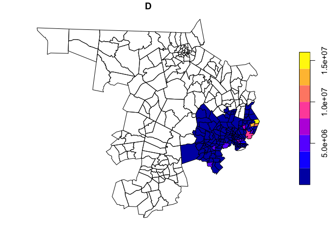

Of course, we may also be interested not only in disinvestment, but in areas of concentrated and racialized affluence (for a discussion of so-called ‘Racially and Ethnically Concentrated Areas of Affluence’, as a response to the more common, damage-focused ‘Racially and Ethnically Concentrated Areas of Poverty’, see Goetz et al. 2019 in Cityscape and Shelton 2018 in Urban Geography).

plot(holc_areas['A'])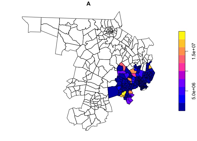

We’ve done a huge amount of spatial processing and data formatting in very little code. Getting comfortable with piping and sf workflows in R will really speed your analysis and, with a little bit of practice, writing these scripts will start to come more easily.

References