Python as a GIS: Public Tree Densities in Cambridge-Somerville

Eric Robsky Huntley, PhD (They/them)
- Lecturer in Urban Science and Planning
- ehuntley@mit.edu
Tutorial Information
- Module 6 in Spatial Data Science.
Methods
Tools
In this workshop, we’ll be using Python’s GeoPandas package to map ‘public’ tree densities in Cambridge and Somerville. This is a fairly straightforward way into spatial analysis using Python, and it has the advantage of being built on top of Pandas, which is a very well-known and well-supported data analysis and manipulation library. There are other ways to do spatial work in Python. In fact, both ArcGIS and QGIS have Python bindings, PyQGIS and ArcPy, respectively!
Indeed, my Very Rigorously Tested (i.e., largely unfounded) theory is that GeoPandas has been relatively slow to arrive because spatial work has long been supported in Python through bindings to the dominant GIS packages. However, given the ascendancy of ‘data science’ as a discipline, discourse, and object of investment (and the concurrent rise of Python as the go-to, can-do language for absolutely everything), it’s useful to not have to leave the comfort of Pandas to work spatially. Furthermore, I (for one) find its ‘way of thinking’ a bit more palatable than PyQGIS or ArcPy, as it is built to behave like Pandas (which is built to behave like R), instead of the Desktop Python bindings (that are built to behave like a Desktop GIS).
Anyway, the point is that today, we’ll be covering how to use GeoPandas to quickly and painlessly write replicable code for spatial analysis in an idiom that is familiar to data analysts (and should be fairly simple for anyone else).
Create a New Virtual Environment
We begin by creating a new virtual environment for our Python spatial work. As a reminder, a virtual environment is a self-contained Python environment, generally built to accommodate a specific project. We use these so that we’re not endlessly installing pacakges into a single bloated environment; instead, we work only with those packages we need.
First, we want to navigate to the folder to which we downloaded the exercise data. In a terminal (macOS/Linux) or command prompt (Windows) window type…
cd path/to/your/data/Once you’ve changed your working directory, you’ll want to create a
new virtual environment using the venv utility, which is a
module (hence, -m) of Python.
# Tells python 3 to run the venv module...
# ...and create a new virtual environment...
# ...in our current directory.
python3 -m venv venv/

# On Windows...
python -m venv venv\
We can activate this virtual environment by running the following at the terminal:
# On macOS or Linux...
. venv/bin/activate
# On Windows...
venv\Scripts\activate.bat
# The next line of your prompt should begin (venv)
Once we’ve activated our virtual environment, any packages we install
will be specific to this environment—this is very useful for managing
packages on a project-by-project basis. We’re going to install the
GeoPandas package, which extends the ever-popular Pandas
package. We’ll also make sure that matplotlib and
descartes are installed (these packages help us plot, in
general, and plot polygons, specifically). We’ll also install
rtree which allows for spatial indexing… without getting
technical, we can say that spatial indexing makes spatial queries a
great deal faster. Finally, we install jupyter, a package
which allows us to develop Python code using code blocks within a
notebook (a very common way to write code that supports written
documentation alongside code chunks).
pip install geopandas matplotlib descartes rtree jupyterFrom your terminal, type…
jupter notebookClick the ‘new’ dropdown on the top right, and select ‘Python 3 (ipykernel)’ to create a new notebook that uses the environment we just built.
Who will Speak for the Trees?
As described above, our goal today is to make a map of tree densities in Cambridge-Somerville by both area of grid cell and land area (excluding water). I’ve provided all the data you’ll need—we begin by importing the public tree datasets from the Cambridge Public Works and the City of Somerville Urban Forestry Division. Note that these are managed by different entities and, as such, we should not make too much of inter-municipal differences in the datasets, as these could simply be artifacts of data collection and classification practices. However, we know that in both cases, they represent trees that are in some way ‘public’, which is to say managed or owned by their respective cities. So this is our universe—‘public’ trees in Cambridge and Somerville.
Importing spatial data looks fairly Pandas-esque! We can use the
read_file function to read the Shapefiles I provided and
inspect the first few rows using the object’s head
method…
import geopandas as gpd
import pandas as pd

cambridge_trees = gpd.read_file('data/cambridge_trees.shp')
cambridge_trees.head()| created | modified | trunks | SiteType | |
|---|---|---|---|---|
| 0 | 2005-09-22 | 2016-08-12 | 1 | Tree |
| 1 | 2005-09-22 | 2016-08-12 | 1 | Tree |
| 2 | 2005-09-22 | 2016-08-12 | 1 | Tree |
| 3 | 2005-09-22 | 2016-08-12 | 1 | Tree |
| 4 | 2005-09-22 | 2016-08-12 | 1 | Tree |
GeoPandas provides an interface to matplotlib that
allows us to make very quick, simple maps. For example, we can plot the
Cambridge trees like so…
cambridge_trees.plot(markersize=0.01, color='green')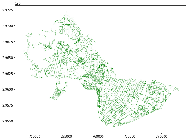
We can read the Somerville trees in the same way…
somerville_trees = gpd.read_file('data/somerville_trees.shp')
somerville_trees.head()| Address | Suffix | Street | Side | |
|---|---|---|---|---|
| 0 | 34 | None | NORTH ST | Side |
| 1 | 61 | None | NORTH ST | Side |
| 2 | 62 | None | NORTH ST | Front |
| 3 | 68 | None | NORTH ST | Front |
| 4 | 71 | None | NORTH ST | Side |
And plot them in the same way!
somerville_trees.plot(markersize=0.01, color='green')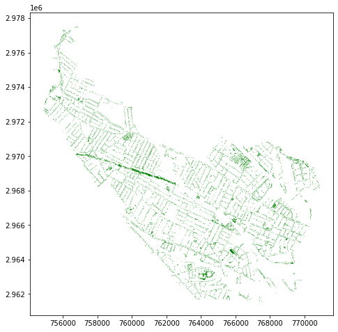
In each case, we get a huge number of variables… inconveniently, the schemas are quite different! Feel free to consult the documentation for Cambridge or Somerville. However, we know that both datasets represent trees that are in some way ‘public’—managed or owned by the respective municipalities—though this might be defined differently in each case.
For simplicity’s sake, today, let’s remove columns that are not the geometry…
cambridge_trees = cambridge_trees[['geometry']]
somerville_trees = somerville_trees[['geometry']]
We’ll also want to merge the two datasets so that we can analyze the Camberville Urban Forest in one go… but let’s think about this. If we’re going to combine spatial datasets, we’re going to want to make sure that our datasets are in the same coordinate reference system (CRS, or projection to use language that might be more familiar to GIS users). If they are not, we’ll be mixing incommensurable coordinates! We can check on the coordinate reference systems for our data like this…
cambridge_trees.crs == somerville_trees.crsTrueSo they match! But we might also want to check the appropriateness of
the CRS. We can ascertain in which CRS our data are stored by
accessing its .crs property.
cambridge_trees.crs<Projected CRS: EPSG:2249>
Name: NAD83 / Massachusetts Mainland (ftUS)
Axis Info [cartesian]:
- X[east]: Easting (US survey foot)
- Y[north]: Northing (US survey foot)
Area of Use:
- name: USA - Massachusetts - SPCS - mainland
- bounds: (-73.5, 41.46, -69.86, 42.89)
Coordinate Operation:
- name: SPCS83 Massachusetts Mainland zone (US Survey feet)
- method: Lambert Conic Conformal (2SP)
Datum: North American Datum 1983
- Ellipsoid: GRS 1980
- Prime Meridian: GreenwichSo we know that our datasets are stored in NAD / Massachusetts
Mainland (ftUS), A.K.A. EPSG:2249. As always, for a CRS
reference, I recommend that you check out epsg.io—the
entry for EPSG:2249 is here. As such, we can append our two
GeoDataFrames withour fear. We use the GeoDataFrame’s
append method to bind somerville_trees to
cambridge_trees and assign it to the new object
trees.
trees = pd.concat([cambridge_trees, somerville_trees])
trees.plot(markersize=0.01, color='green')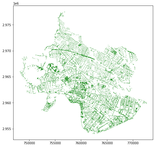
I belabor the point about projections because GeoPandas
does woefully little to keep you on the right track.
Aggregate to Hexagons
In order to analyze tree density, we’re going to aggregate trees to a
regular grid. I’ve provided a shapefile that includes regular
hexagonal bins. You may remember from a previous workshop that R
provides a very tidy means by which to do this: namely the
st_make_grid() function of the sf package.
GeoPandas is less full-featured. I’ve written unction that will generate
a regular rectangular or hexagonal grid over an arbitrary extent given a
cell size—this is included at the end of this tutorial. Feel free to use
my efforts in your own work! But walking through that function is
outside of the scope of this workshop.
You may ask: why hexagons? Good question! Geographers love hexagons. Why do geographers love hexagons? Glad you asked.
Basically, it’s because…
- Unlike a square grid, the distance from the center of a hexagon to its edge is approximately constant and
- unlike a grid of radial distnaces (circles) cells in an exhaustive grid of hexagons do not overlap.
Expanding on point 1: for a square, $ d_{orthoganal} = d_{diagonal} $, where $ d_{orthogonal} $ is the distance from the center of the square to its edge along an orthoganal angle and $ d_{diagonal} $ is the distance from the center of the square to any given corner. This means that the distance from a grid center to its associated points can vary. A circle would fix this problem, but try making a grid of circles… they’ll overlap if you try to make them exhaustively cover the study area.
So let’s read in our hexagons and aggregate our trees to their extents.
hex_bins = gpd.read_file('data/hex_bins.shp')Now, this starts to look quite a bit like a normal GIS workflow.
We’re going to count points in polygons, which is a combination of a
spatial join (to impute the hexagon id to the trees), and a
dissolve on the hexagon id. Most GIS platforms do this for
you in one step, but GeoPandas (and sf for that matter) will make you do
it in a couple of steps.
First we create a new object called tree_count and store
the result of a inner spatial join between
trees and hex_bins. inner here
refers to an inner join, or a join that preserves only tree that meet
the spatial criteria—namely that they intersect geometries
in the second/right table. The result of this is a table with the tree
POINT geometry and the index position of the right table
and its id column (in this case, these are the same).
tree_count = gpd.sjoin(trees, hex_bins, how='inner', predicate='intersects')
tree_count.head()| geometry | index_right | id | |
|---|---|---|---|
| 0 | POINT (759827.721 2965044.675) | 296 | 296 |
| 1 | POINT (759787.376 2965047.192) | 296 | 296 |
| 2 | POINT (759609.651 2965054.781) | 296 | 296 |
| 3 | POINT (759518.862 2965060.663) | 296 | 296 |
| 4 | POINT (759463.213 2965064.087) | 296 | 296 |
This is maybe easier to visualize… let’s map it.
tree_count.plot(column='id', markersize=0.01)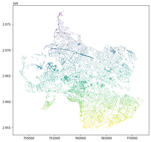
On this map, we can see that each tree has been imputed with the id
integer value of the hexagon within which it sits. Now, to count this
information, we can dissolve the trees by the hexagon
id—this will perform an aggregate statistic on all trees
associated with each hexagon id. We simply want to
count them, but we could also calculate a range of other
summary statistics (mean, median, etc.) but
these would be meaningless for an index position.
tree_count = tree_count.dissolve(by='id', aggfunc='count')
tree_count.head()| geometry | index_right | |
|---|---|---|
| id | ||
| 7 | MULTIPOINT (755923.238 2976924.853, 755925.242… | 57 |
| 8 | MULTIPOINT (756697.642 2977473.398, 756719.326… | 8 |
| 28 | MULTIPOINT (755500.105 2976294.267, 755500.962… | 55 |
| 29 | MULTIPOINT (755951.344 2976628.684, 755969.723… | 54 |
| 51 | MULTIPOINT (755438.915 2975707.363, 755476.594… | 110 |
We can see that we’ve now calculated the count of trees in in each
hexagon cell! Let’s tidy up our table a bit, renaming the
index_right column to tree_count, and dropping
the geometry column—we’re going to join this count to our original
hexagonal data for visualization, so the MULTIPOINT
geometries we’ve created for each cell aren’t terribly useful.
tree_count = tree_count.rename({'index_right': 'tree_count'}, axis='columns')
tree_count = tree_count.drop(columns='geometry')
tree_count.head()| tree_count | |
|---|---|
| id | |
| 7 | 57 |
| 8 | 8 |
| 28 | 55 |
| 29 | 54 |
| 51 | 110 |
We can then use the merge method to merge the
hex_bins with the tree_count. We merge on
id in both the left and the right table (the
hex_bins and the tree_count, respectively). We
specify a left join! This retains even those hexagons in
which there are no matching rows in the tree_count table
(i.e., those hex cells in which there were no trees).
hex_bins = hex_bins.merge(tree_count, left_on='id', right_on='id', how='left')Samplign the results, we see that, indeed, our hex_bins
table now includes the tree_count column. We can also map it,
visualizing based on the tree_count column to see our
aggregate data.
hex_bins.head()| id | geometry | tree_count | |
|---|---|---|---|
| 0 | 0 | POLYGON ((748154.000 2978173.801, 748710.682 2… | NaN |
| 1 | 1 | POLYGON ((749267.364 2978173.801, 749824.045 2… | NaN |
| 2 | 2 | POLYGON ((750380.727 2978173.801, 750937.409 2… | NaN |
| 3 | 3 | POLYGON ((751494.091 2978173.801, 752050.773 2… | NaN |
| 4 | 4 | POLYGON ((752607.455 2978173.801, 753164.136 2… | NaN |
hex_bins.plot(column='tree_count')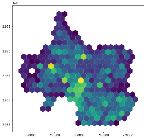
Accounting for Spatial Heterogeneity
One of the reasons regular grids are appealing is because counts within a regular grid are already, implicitly, a density. The visualization above is giving us counts per cell, yes, but because each cell has the same area, we’re also implicitly seeing a visualization of counts per area. But this can be (and often is!) misleading! Urban space is heterogeneous. Densities of trees are likely to be affected by how much of each give area is open space, how much is included in a campus, and (maybe most obviously) how much of a given hex cell’s area is not land at all, but is instead covered by a water body.
We’ll first satisfy ourselves that our polygons do indeed have the same areas.
hex_bins['area'] = hex_bins.geometry.area
hex_bins.head()| id | geometry | tree_count | area | |
|---|---|---|---|---|
| 0 | 0 | POLYGON ((748154.000 2978173.801, 748710.682 2… | NaN | 1.073507e+06 |
| 1 | 1 | POLYGON ((749267.364 2978173.801, 749824.045 2… | NaN | 1.073507e+06 |
| 2 | 2 | POLYGON ((750380.727 2978173.801, 750937.409 2… | NaN | 1.073507e+06 |
| 3 | 3 | POLYGON ((751494.091 2978173.801, 752050.773 2… | NaN | 1.073507e+06 |
| 4 | 4 | POLYGON ((752607.455 2978173.801, 753164.136 2… | NaN | 1.073507e+06 |
hex_bins.plot(column='area')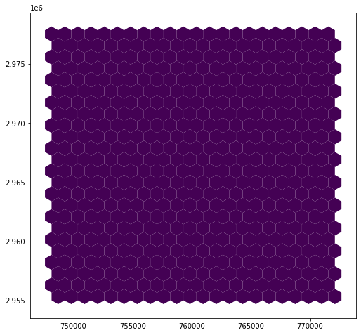
Indeed. Each cell has an area of 1.073507e+06 square feet. We know the units because the units are going to match the unit of our data layer’s projection (in this case US feet). This means we can also convert to square miles trivially, using a conversion factor. One square mile equals 2.788e+7 square feet, so…
hex_bins['area_sqmi'] = hex_bins.area / 2.788e+7
hex_bins.head()| id | geometry | tree_count | area | area_sqmi | |
|---|---|---|---|---|---|
| 0 | 0 | POLYGON ((748154.000 2978173.801, 748710.682 2… | NaN | 1.073507e+06 | 0.038505 |
| 1 | 1 | POLYGON ((749267.364 2978173.801, 749824.045 2… | NaN | 1.073507e+06 | 0.038505 |
| 2 | 2 | POLYGON ((750380.727 2978173.801, 750937.409 2… | NaN | 1.073507e+06 | 0.038505 |
| 3 | 3 | POLYGON ((751494.091 2978173.801, 752050.773 2… | NaN | 1.073507e+06 | 0.038505 |
| 4 | 4 | POLYGON ((752607.455 2978173.801, 753164.136 2… | NaN | 1.073507e+06 | 0.038505 |
But not all of this area is land area. Let’s account for
this using water geometries pulled from the U.S. Census! (This is the
2019 TIGER/Line Water Shapefile for both Suffolk and Middlesex
counties.) We read and plot it, as we’ve been doing, while layering it
on top of the hex_bins.
water = gpd.read_file('data/water.shp')
hex_map = hex_bins.plot(column='tree_count')
water.plot(ax=hex_map, color='red')
Aha! Looks like we have a projection issue. Examining our projections, we see that they do not match; the water layer is presented in EPSG:4326 (WGS84).
print(hex_bins.crs, water.crs)epsg:2249 epsg:4326We can reproject the water trivially using the to_crs
method; furthermore, we can put some controls on the process by simply
reading the crs directly from hex_bins.
water = water.to_crs(hex_bins.crs)hex_map = hex_bins.plot(column='tree_count')
water.plot(ax=hex_map, color='red')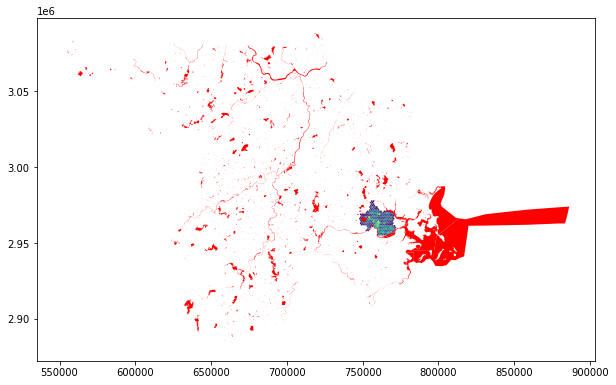
Better! Out water bodies now overlap with our hexagons… we’ll next
need to perform a geometric intersection to determine how much of each
hexagon is within a water body. Such an intersection is one of several
overlay operations supported by GeoPandas. Mapping the
result, we see that our results are a polygon feature set that includes
only those areas that overlapped between the hex grid cells and the
water features.
hex_bins_water = gpd.overlay(hex_bins, water, how='intersection')
hex_bins_water.plot()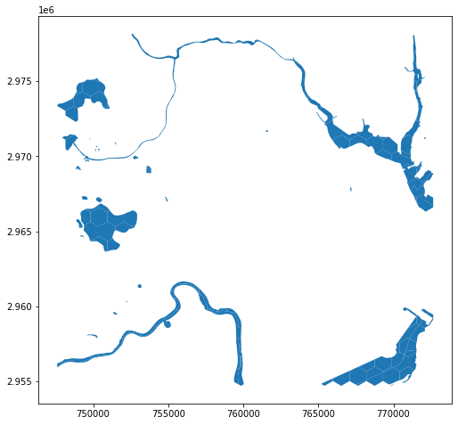
hex_bins_water.head()| id | tree_count | area | area_sqmi | ANSICODE | HYDROID | FULLNAME | MTFCC | ALAND | AWATER | INTPTLAT | INTPTLON | geometry | |
|---|---|---|---|---|---|---|---|---|---|---|---|---|---|
| 0 | 4 | NaN | 1.073507e+06 | 0.038505 | None | 1105590176101 | None | H2030 | 0 | 135377 | +42.4145431 | -71.1324976 | POLYGON ((752607.455 2978173.801, 752670.164 2… |
| 1 | 5 | NaN | 1.073507e+06 | 0.038505 | None | 1105590176101 | None | H2030 | 0 | 135377 | +42.4145431 | -71.1324976 | POLYGON ((753333.348 2977111.905, 753164.136 2… |
| 2 | 7 | 57.0 | 1.073507e+06 | 0.038505 | None | 1105590176101 | None | H2030 | 0 | 135377 | +42.4145431 | -71.1324976 | POLYGON ((756504.227 2977570.710, 756504.227 2… |
| 3 | 8 | 8.0 | 1.073507e+06 | 0.038505 | None | 1105590176101 | None | H2030 | 0 | 135377 | +42.4145431 | -71.1324976 | POLYGON ((756504.227 2977486.531, 756504.227 2… |
| 4 | 26 | NaN | 1.073507e+06 | 0.038505 | None | 1105590176101 | None | H2030 | 0 | 135377 | +42.4145431 | -71.1324976 | POLYGON ((753164.136 2977209.600, 753333.348 2… |
We also have all attributes from both tables. This is excessive! All
we really need are the hexagon id (id) and the intersected
hexagon-hydrology geometry (geometry). Our tree counts and
hexagon areas are stored on the original hex_bins object,
so we can drop them. The areas depicted here also no longer correspond
to the polygons to which they’re tied, which might be somewhat
confusing! For our sanity, let’s cull our fields.
hex_bins_water = hex_bins_water.loc[:,['id', 'geometry']]We can now calculate the area for these intersected polygons in the same manner as above…
hex_bins_water['water_area'] = hex_bins_water.geometry.area
hex_bins_water['water_area'] = hex_bins_water.area
And dissolve in the same manner as above… except here we’re summing the area, rather than counting. To test your own understanding: what would counting give us a count of?
hex_bins_water = hex_bins_water.dissolve(by='id', aggfunc='sum')hex_bins_water.head()| geometry | water_area | |
|---|---|---|
| id | ||
| 4 | POLYGON ((752607.455 2978173.801, 752670.164 2… | 111090.885902 |
| 5 | POLYGON ((753333.348 2977111.905, 753164.136 2… | 11486.988249 |
| 7 | POLYGON ((756504.227 2977570.710, 756504.227 2… | 104026.764360 |
| 8 | POLYGON ((756504.227 2977486.531, 756504.227 2… | 94817.529307 |
| 9 | POLYGON ((758730.955 2977621.302, 758730.955 2… | 159173.524828 |
Let’s now drop the geometry and merge the table with our
hex_bins!
hex_bins_water = hex_bins_water.drop(columns='geometry')
hex_bins = hex_bins.merge(hex_bins_water, left_on='id', right_on='id', how='left')
hex_bins.head()| id | geometry | tree_count | area | area_sqmi | water_area | |
|---|---|---|---|---|---|---|
| 0 | 0 | POLYGON ((748154.000 2978173.801, 748710.682 2… | NaN | 1.073507e+06 | 0.038505 | NaN |
| 1 | 1 | POLYGON ((749267.364 2978173.801, 749824.045 2… | NaN | 1.073507e+06 | 0.038505 | NaN |
| 2 | 2 | POLYGON ((750380.727 2978173.801, 750937.409 2… | NaN | 1.073507e+06 | 0.038505 | NaN |
| 3 | 3 | POLYGON ((751494.091 2978173.801, 752050.773 2… | NaN | 1.073507e+06 | 0.038505 | NaN |
| 4 | 4 | POLYGON ((752607.455 2978173.801, 753164.136 2… | NaN | 1.073507e+06 | 0.038505 | 111090.885902 |
Examining the resulting table, we can see that many of our cells have no area that includes water. Earlier, for our tree count, we left these as NaN because the preponderance of them were outside the ‘study area’, which means that they are truly missing values, not zero measurements. These things are conceptually different! But in the case of the water_area, we know that these are truly zeros (or as ‘truly’ as is permitted by our data set).
Furthermore, this is going to cause some practical problems! Let’s
try to calculate our land area by subtracting the
water_area from the area.
hex_bins['land_area'] = hex_bins.area - hex_bins.water_area
hex_bins.plot(column='land_area')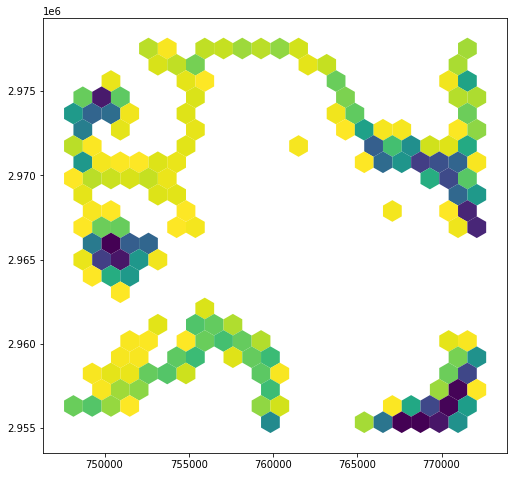
In cases where water_area is NaN, the
land_area is also NaN! Meaning that cells with
100% land area appear to be unmeasured. As such, let’s replace
NaN values with zeroes in the water_area
column.
values = {'water_area': 0}
hex_bins = hex_bins.fillna(value=values)
hex_bins.head()| id | geometry | tree_count | area | area_sqmi | water_area | land_area | |
|---|---|---|---|---|---|---|---|
| 0 | 0 | POLYGON ((748154.000 2978173.801, 748710.682 2… | NaN | 1.073507e+06 | 0.038505 | 0.000000 | NaN |
| 1 | 1 | POLYGON ((749267.364 2978173.801, 749824.045 2… | NaN | 1.073507e+06 | 0.038505 | 0.000000 | NaN |
| 2 | 2 | POLYGON ((750380.727 2978173.801, 750937.409 2… | NaN | 1.073507e+06 | 0.038505 | 0.000000 | NaN |
| 3 | 3 | POLYGON ((751494.091 2978173.801, 752050.773 2… | NaN | 1.073507e+06 | 0.038505 | 0.000000 | NaN |
| 4 | 4 | POLYGON ((752607.455 2978173.801, 753164.136 2… | NaN | 1.073507e+06 | 0.038505 | 111090.885902 | 962415.660234 |
Recalculating our land area, we now see results that make more sense…
hex_bins['land_area'] = hex_bins.area - hex_bins.water_area
hex_bins.plot(column='land_area')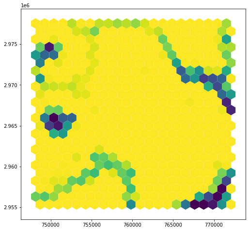
We can now calculate the number of trees per land area!
hex_bins['land_area_sqmi'] = hex_bins.land_area / 2.788e+7
hex_bins['trees_p_sqft'] = hex_bins['tree_count'] / hex_bins['land_area']
hex_bins['trees_p_sqmi'] = hex_bins['tree_count'] / hex_bins['land_area_sqmi']
hex_bins.plot(column='trees_p_sqmi')
Wrapping Up…
Now that we’ve performed this (replicable, self-documenting!-ish)
procedure, we can export our GeoDataframe as a Shapefile or
a GeoJSON for use in a Desktop GIS, a web map, or any other purpose you
can think of. This is a simple matter of writing…
hex_bins.to_file('trees_p_area.shp')
hex_bins.to_file('trees_p_area.geojson', driver='GeoJSON')
hex_bins.to_file('trees_p_area.gpkg', driver='GPKG')
Appendix: Generating the Hex…
As I pointed out above, the spatial ecosystem for Python is much less
well-developed than the ecosystem for R. GeoPandas, while promising,
does not have all of the functionality found in, say, R’s
sf package. One of the functions that sf
provides that is frustratingly absent in GeoPandas is the
ability to automatically generate a hexagonal or square grid over an
area. But, not to fear! This is such a common task that I’ve put
together a function that you can use to generate regular square and
hexagonal grids. It accepts a GeoDataFrame or
GeoSeries whose extent will be the extent of the grid; a
cell size (in the units of the Geo* object’s CRS); and a
buffer value, measured as a proportion of the total width and height
dimensions. This function is based on code by Navaneeth
Mohan, though I’ve extended it and corrected some of their
errors.
To generate the hexagon grid and export it for the above exercise, I simply ran…
hex_bins = make_grid(geo = trees, size = 1320, hexagon = True, buffer = 0)
hex_bins.to_file('hex_bins.shp')
import numpy as np
from math import ceil
from matplotlib.patches import RegularPolygon
from shapely.geometry import Polygon, box
def make_grid(geo, size, hexagon=False, buffer=False):
# Diameter of each hexagon
d = size
if hexagon:
# Horizontal width of each hexagon
w = d * np.sin(np.pi/3)
else:
w = size
bbox = geo.total_bounds
xmin, ymin, xmax, ymax = bbox
xmin = int(np.floor(xmin))
xmax = int(np.ceil(xmax))
ymin = int(np.floor(ymin))
ymax = int(np.ceil(ymax))
tot_width = xmax - xmin
tot_height = ymax - ymin
if buffer:
xmin = int(np.floor(xmin - (buffer * 0.5 * tot_width)))
ymin = int(np.floor(ymin - (buffer * 0.5 * tot_height)))
xmax = int(np.floor(xmax + (buffer * 0.5 * tot_width)))
ymax = int(np.floor(ymax + (buffer * 0.5 * tot_height)))
tot_width = xmax - xmin
tot_height = ymax - ymin
if hexagon:
# Number of cells (hexagons) per row
n_cols = int(np.ceil(tot_width / w))
else:
# Number of cells per row.
n_cols = int(np.ceil(tot_width / d))
# Number of cells per column.
n_rows = int(np.ceil(tot_height / (d * 0.75)))
print(d, w)
grid = []
w = tot_width / n_cols
if hexagon:
d = w / np.sin(np.pi/3)
for row in range(0, n_rows):
for col in range (0, n_cols):
x = xmin + (col * w)
if (row % 2) == 1:
x = x + w / 2
y = ymax - (row * d * 0.75)
hexpoly = RegularPolygon((x,y), numVertices=6, radius=d/2)
trans = hexpoly.get_patch_transform()
verts = hexpoly.get_path().vertices
points = trans.transform(verts)
grid.append(Polygon(points))
else:
h = tot_height / n_rows
for row in range(0, n_rows):
for col in range(0, n_cols):
x = xmin + (col * w)
y = ymax - (row * h)
grid.append(box(x, y-w, x+w, y))
gdf = gpd.GeoDataFrame({'geometry': grid}, crs=geo.crs)
gdf['id'] = gdf.index
return(gdf)