Mapping Social Space: Networks and Relations

In Massachusetts, we benefit from an unusually robust public entity that concerns itself with managing spatial data statewide - this is the Bureau of Geographic Information, or MassGIS. It’s worth taking some time to familiarize yourself with the many layers MassGIS makes available to you, but today, we’re focusing specifically on its statewide Property Tax Parcel database. This is collected from assessor’s offices around the state and contains a vast (though inconsistently complete) body of information about properties and structures built on them.

While it’s possible to download the whole state at once, that involves gigabytes of information and millions of rows - properly big data, which is quite cumbersome. Instead, let’s focus on Chelsea, MA, a ‘gateway city’ just north of Boston. Specifically, let’s look into the ownership of Chelsea’s industrial landscape.

You can download Chelsea data from the interactive map interface available here. (While you’re here, note one of the data set’s major inconsistencies: the last reported fiscal year for each municipality varies!)

Join Assessor’s Tables

Once you’ve downloaded and extracted the data, you’ll see that there are many available layers and data tables (.dbf files). We’re specifically interested in M05TaxPar_CY22_FY23—these are the parcels themselves—and M057Assess_CY22_FY23.dcf—this is a table of assessors information related to each property. Add the tax parcels.

Open the attribute table - most of this information relates to the parcel itself, not its assessment. We need to join the assessor’s database! Drag the assessing table into the project (it won’t look like anything happened on the map). Next, right-click the parcel layer, open its properties, and select Joins > Add. Your join layer is the assessors table (M057Assess...). You want to join based on the LOC_ID field in both tables - this a unique parcel identifier shared by both tables that we use to associate assessing data with the tax parcel.

Open the attribute table: you should see a vastly expanded collection of columns, including land use (USE_CODE), assessed value (TOTAL_VAL), and (much) more. We also have information about the property’s owner: see the OWNER1, OWN_ADDR, OWN_CITY, OWN_STATE, OWN_ZIP. This is the information we’ll use to locate the owners using geocoding.

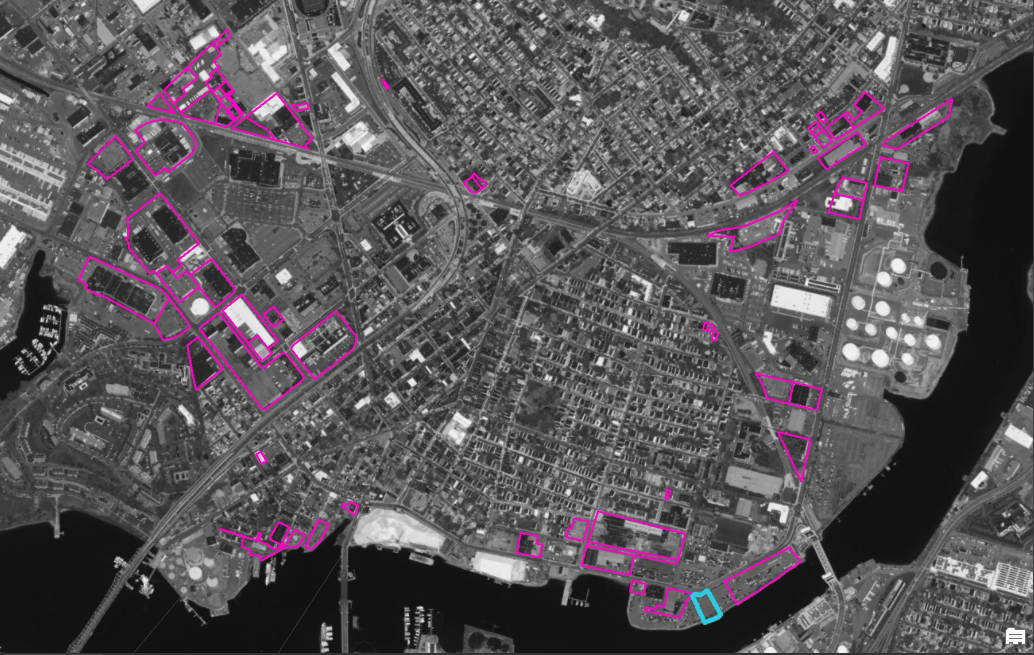
But first, let’s subset our parcels to include only those that have an industrial land use, broadly defined.

Identify Manufacturing Parcels

Massachusetts uses a very comprehensive state land use code, maintained by the Department of Revenue. The code looks like this:

We want to query the layer for all codes related to industrial uses. We’ll do this by clicking ‘select by attributes’ and building a query that returns parcels with land use codes between 400-404, 410-413, 420-426, and 450-452. In SQL, this looks like this:

-- Return all USE_CODE starting with 40, etc.
a_USE_CODE LIKE '40%' Or
a_USE_CODE LIKE '41%' Or
a_USE_CODE LIKE '42%' Or
a_USE_CODE LIKE '45%'

Note my use of the % ‘wildcard’, which can be replaced with any number of characters. This keeps me from having to write out each query separately.

Right-click the layer and choose Export > Save Selected Features As. Save it as a new shapefile.

Finally, right-click that new layer and select Export > Save Features As. Export the table to a CSV without its geometry - we’ll need this for geocoding.

Geocode Owners

Now, we’ll find the owners of these parcels! If you haven’t already, install the MMQGIS plugin for QGIS. Your input table is the industrial parcel table you just exported. Use the OpenStreetMap/Nominatim service which is the geocoding service that OSM built for its web application. The address is OWN_ADDR. The city is OWN_CITY. The State is OWN_STATE, and the country is OWN_CO. Save it to a new shapefile.

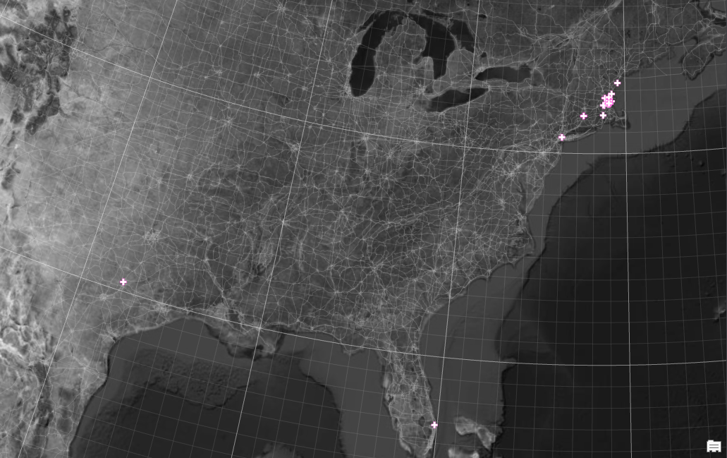
This will take a little while— this is probably not the best solution for a large number of records. To built a better geocoder, check out this tutorial. When it’s done, you’ll see points appear both in Chelsea and far outside of it.

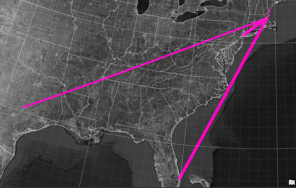
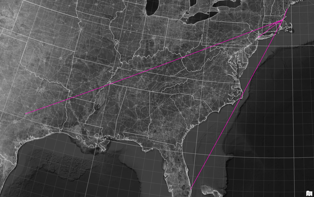
Generate Origin-Destination Links

Now, we’ll build what’s sometimes called a ‘spider diagram’ (or, my preferred term, a ‘🍝 map’ - that’s spaghetti). To do this, we’ll join these new-found owner locations to the parcel locations.

We want to use the Join by Lines (hub lines) tool to produce origin-destination links between owners and parcels. Link your parcels (your hub layer) to your owner locations (your spoke layer). In both cases, your ID field is LOC_ID - this is functionally like the join operation we did above. Run the operation.

We get something like this:

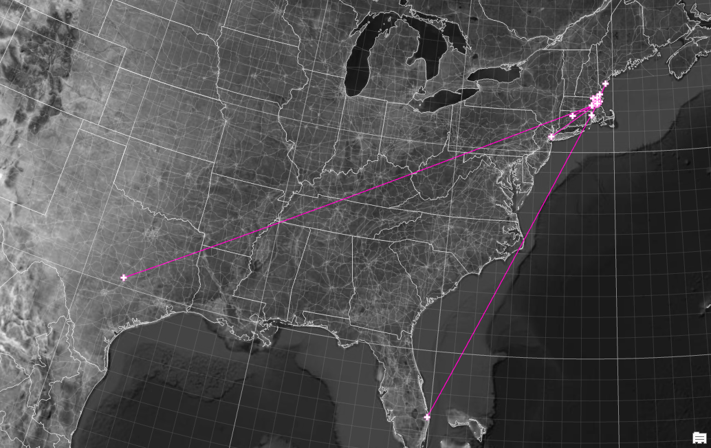
Visualize Using Assessing Information

We can use any of the assessor’s table variables to visualize these lines by e.g., assessed value, etc. For example, we could use a display filter to only show those locations outside of Massachusetts:

Or to size the line by assessed value:

References