Mapping in R: Street Trees in Cambridge-Somerville

Read Data

We begin by reading the tree census data I’ve provided. These are two separate shapefiles, so we will read them independently using the st_read function. Both contain quite a bit of potentially useful information about each surveyed tree—especially Cambridge, whch provides a full 60 attributes! However, for our simple analysis today, we’re going to satisfy ourselves with each tree’s point location, stored in the ‘geometry’ column of each layer.

require('sf')
require('dplyr')
require('tibble')

cambridge_trees <- st_read('data/cambridge_trees.shp') %>%
  select(c('geometry'))

somerville_trees <- st_read('data/somerville_trees.shp') %>%
  select(c('geometry'))

With this single column selected, we can elect to combine the two using the rbind function to bind the sf objects by row (hence,r). Plotting the trees, we see a street canopy that hews quite closely to what we know to be Cambridge-Somerville’s built form.

trees <- rbind(cambridge_trees, somerville_trees)
plot(trees, pch='.', col='green')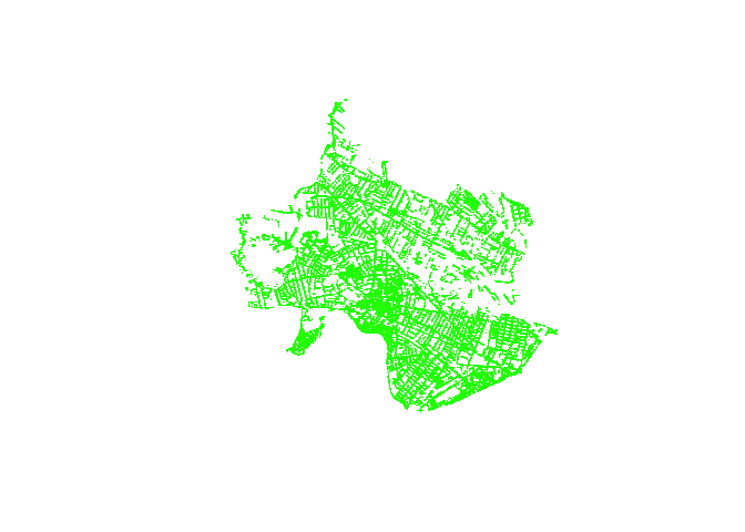

Generate Hex Grid

We now want to generate a grid of consistently-sized cells over which to evaluate the density of street trees in Cambridge-Somerville. Specifically, we want to generate a hexagonal grid.

Geographers love hexagons! This is because the distance from the center of a hexagon to its edge is approximately constant. This means that points included in a hexagon are going to be much closer to those that are within a threshold distance. This is not true for a square grid! For a square, $ d_{orthoganal} = d_{diagonal} $, where $ d_{orthogonal} $ is the distance from the center of the square and $ d_{diagonal} $ is the distance from the center of the square to any given corner.

We can use the st_make_grid function to generate a regular hexagonal grid of half-mile cells. square=FALSE instructs the function to generate hexagons. Finally, we convert the simple feature collection (sfc) geometries that are created to an sf object using st_sf and create an id column called hex_id using rowid_to_column().

hex <- st_make_grid(trees, cellsize=2640, square=FALSE) %>%
  st_sf() %>%
  rowid_to_column('hex_id')
plot(hex)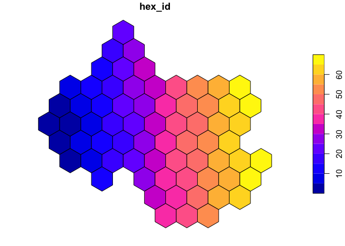

You can, of course, use different cell sizes; in general, you’ll find that larger cell sizes lead to more preditable behavior (tighter clustering around the sample mean, etc.), but that you lose spatial granularity as the cell size increases.

Count Points in Polygons

Now that we’ve created a grid, we can count the number of trees in each polygon quite simply. We perform a spatial join between the trees and the hexbins, using a st_within criterion. This means that trees will be joined to the hexagons within which they fall. We can plot the results and see that each tree has taken on the hex_id of the hexagon within which it falls.

trees_in_hex <- st_join(trees, hex, join=st_within)
plot(trees_in_hex, pch='.')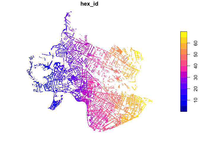

Ultimately, though, we’re not interested in the tree geometries, but in the count per hexagon cell. As such, let’s remove the geometry from the joined table and count the number of trees falling within each cell by grouping on the hex_id. We can do all of this in a single step using dplyr syntax like so…

trees_in_hex <- st_join(trees, hex, join=st_within) %>%
  # Remove geometry.
  st_set_geometry(NULL) %>%
  # County the number of rows per hex_id and 
  # Store this number in a field named 'trees'.
  count(name='trees', hex_id)
head(trees_in_hex)

## # A tibble: 6 x 2
##   hex_id trees
##    <int> <int>
## 1      2    11
## 2      3   131
## 3      4    49
## 4      5   253
## 5      6    14
## 6      7   607

Finally, we can use left_join to join the resulting trees_in_hex table to the hex table, retaining even those cells with no trees. Hexagon cells without any street trees will then have NA values. Let’s replace these with 0s, because we know that these have no recorded street trees—it is not only that values are unknown or missing.

hex <- hex %>%
  left_join(trees_in_hex, by = 'hex_id') %>%
  replace(is.na(.), 0)

plot(hex['trees'])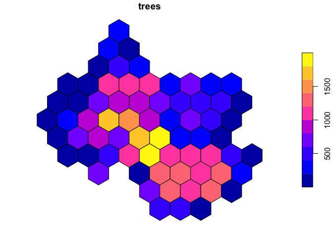

Create a Simple Map

We now have an analytically useful, if simple, dataset! However, those plot functions are quickly reaching the outer edges of their usefulness. Geographic analysis is often an exercise in discerning the relationship between phenomenon and context—said simply, a basemap would be a useful thing to have! Interacting with our maps also becomes quite useful as we begin to explore Cambridge-Somerville’s urban canopy.

For these reasons, the R wrapper for Leaflet is quite a useful thing. Leaflet is one of the most common and usable interative mapping libraries around; the fact that there is now a package that allows us to interface with its functionality without ever leaving R is marvelous. And it’s quite simple to use! Let’s make a first map.

We’ll create a new leaflet object, and—again, using the piping syntax—set its view such that it is centered on Cambridge-Somerville, and such that its view is set to a moderate 13. Map tiles (and therefore web maps) use standard zoom levels from 0-20, where 0 is the least-zoomed-in and 20 is the most.

If we assign our map to a variable name, we can print it by simply invoking the variable name.

require('leaflet')
map <- leaflet() %>%
  setView(lng = -71.111408, lat = 42.38172, zoom = 13) %>%
  addTiles()
map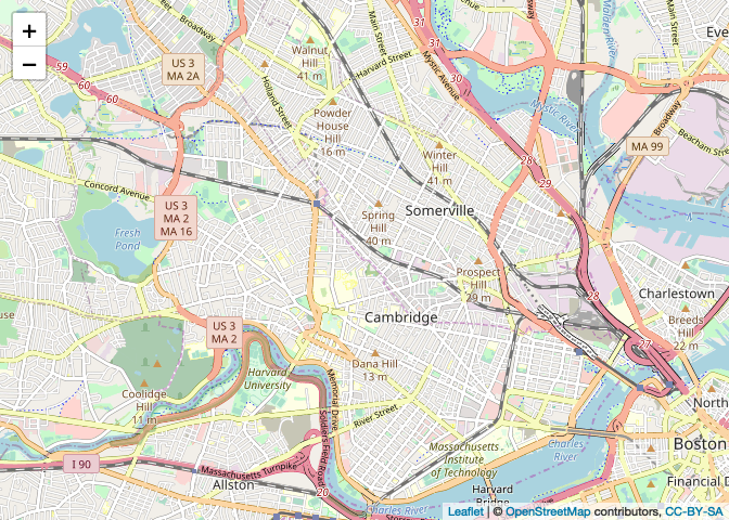

By default, leaflet will use an OpenStreetMap-styled basemap. Nothing wrong with that! After all, most (non-Google, Apple, or Bing) web map tilesets are just styled OpenStreetMap data. But if you want a slightly more stylized basemap, R’s leaflet provides a providers object that lists many available basemap providers. These line up with those made available through the Leaflet providers interface, if you want a slightly more visible way to browse.

providers[1:5]

## $OpenStreetMap
## [1] "OpenStreetMap"
## 
## $OpenStreetMap.Mapnik
## [1] "OpenStreetMap.Mapnik"
## 
## $OpenStreetMap.DE
## [1] "OpenStreetMap.DE"
## 
## $OpenStreetMap.CH
## [1] "OpenStreetMap.CH"
## 
## $OpenStreetMap.France
## [1] "OpenStreetMap.France"

Once you’ve landed on one you like, you can load it using the addProviderTiles function, with the associated tileset name.

map <- leaflet() %>%
  setView(-71.111408, 42.38172, 13) %>%
  addProviderTiles("Stamen.TonerLite")
map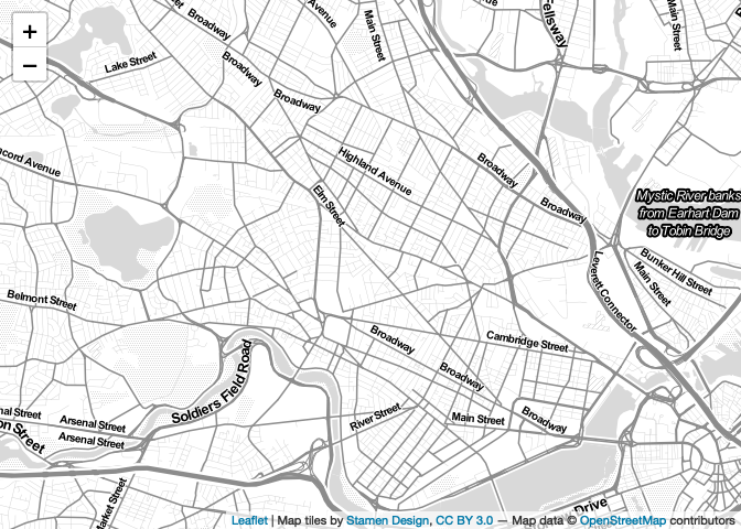

At this point, we’ve included a basemap, but we have yet to include our data. Let’s change that! We begin by passing our hexbins through the leaflet object, and add the geometries by using the addPolygons() function. Notice that the leaflet object knows to create polygons based on the dataset piped to the constructor.

map <- hex %>%
  leaflet() %>%
  setView(-71.111408, 42.38172, 13) %>%
  addProviderTiles("Stamen.TonerBackground")  %>%
  addPolygons()

## Warning: sf layer is not long-lat data

## Warning: sf layer has inconsistent datum (+proj=lcc +lat_1=42.68333333333333 +lat_2=41.71666666666667 +lat_0=41 +lon_0=-71.5 +x_0=200000.0001016002 +y_0=750000 +ellps=GRS80 +towgs84=0,0,0,0,0,0,0 +units=us-ft +no_defs ).
## Need '+proj=longlat +datum=WGS84'

map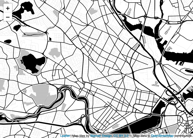

Oh no! Why are we seeing this error?sf layer is not long-lat This is because leaflet expects data that is stored in the WGS 84 coordinate reference system (projection). As demonstrated last week, we can reproject data quite simply using st_transform, and an EPSG code (in this case EPSG:4326).

hex <- st_transform(hex, 4326)

map <- hex %>%
  leaflet() %>%
  setView(-71.111408, 42.38172, 13) %>%
  addProviderTiles("Stamen.TonerBackground")  %>%
  addPolygons()
map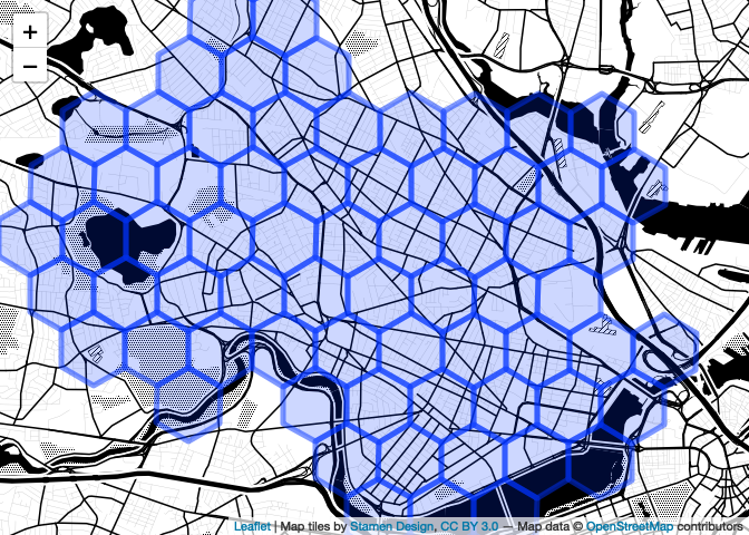

Better! Note that if you don’t like the ‘pipe the data to the leaflet constructor’ syntax I’m using, this is a perfectly fine alternative, which does the same thing and perhaps the reduces the ambiguity.

map <- leaflet() %>%
  setView(-71.111408, 42.38172, 13) %>%
  addProviderTiles("Stamen.TonerBackground")  %>%
  addPolygons(data = hex)
map

Choropleth!

We can extend this code ever-so-slightly to produce a choropleth map that visualizes our street tree counts. We do this using the ColorBin function to create a palette function that will assign a color to each hexagonal cell based on its data value. We pass a color ramp, a domain (i.e., a range of all possible values), and a number of bins. By default, colorBin uses an equal-interval classification scheme.

palette <- colorBin('Greens', domain = hex$trees, bins = 5)
palette(c(400,800, 1250))

## [1] "#EDF8E9" "#BAE4B3" "#74C476"

Greens here refers to the Greens Colorbrewer color ramp… to see all available RColorBrewer color ramps, simply invoke RColorBrewer’s display.brewer.all().

require('RColorBrewer')
display.brewer.all()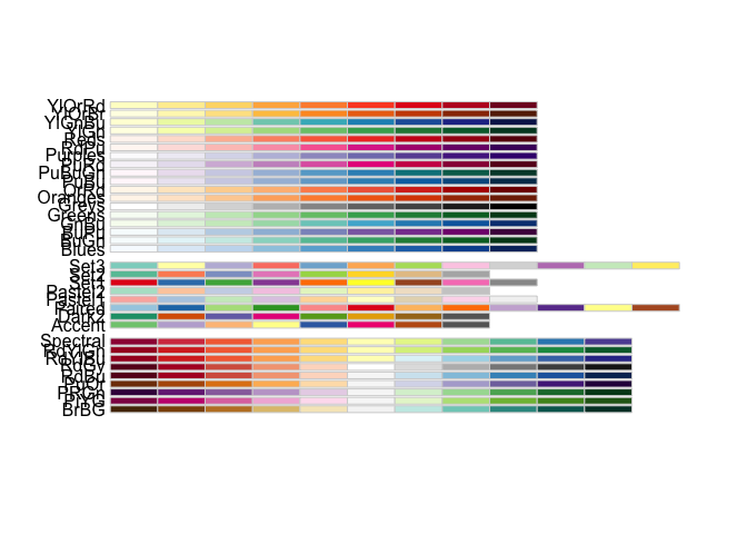

With this new palette in hand, we can modify our addPolygons function call as below. Note that I also begin passing in other style parameters—fillOpacity, opacity (stroke opacity), weight (stroke weight), and color (stroke color).

map <- hex %>%
  leaflet() %>%
  setView(-71.111408, 42.38172, 13) %>%
  addProviderTiles("Stamen.TonerLite")  %>%
  # for each row, assign a fill color based on the 
  # value returned by the palette() function
  addPolygons(
    fillColor = ~palette(trees),
    fillOpacity = 0.7,
    opacity = 1,
    weight = 1,
    color='white'
  )
map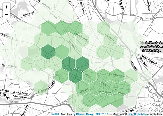

Control Your Class Breaks…

We know, though, that class breaks can have quite a dramatic effect on the interpreting of visualized data. We don’t necessarily want to simply accept an equal intervals scheme and call it a day! It’s good, then, that Jenks natural breaks, quantile breaks, and many others are readily available using the classInt package, which interfaces quite neatly with the ColorBin function.

For example, if we wanted quantiles, broken across seven classes, we would first create the quantile breaks using the classIntervals function with a value of quantile passed to thestyle parameter…

require('classInt')
quantiles <- classIntervals(hex$trees, n=7, style='quantile')
print(quantiles)

## style: quantile
##   one of 74,974,368 possible partitions of this variable into 7 classes
##        [0,129.2857) [129.2857,223.5714) [223.5714,481.2857) [481.2857,660.7143) [660.7143,923.4286) [923.4286,1186.286)     [1186.286,1974] 
##                  10                  10                  10                   9                  10                  10                  10

print(quantiles$brks)

## [1]    0.0000  129.2857  223.5714  481.2857  660.7143  923.4286 1186.2857 1974.0000

Note that this function returns a few different variables—we’re interested in its brks, which is a list of values that form break points for our classification scheme. We can then pass this to the bins parameter of colorBin.

palette_quantiles <- colorBin('Greens', domain = hex$trees, bins=quantiles$brks, pretty=FALSE)

We can then modify our map to use this palette instead of the default palette.

map <- hex %>%
  leaflet() %>%
  setView(-71.111408, 42.38172, 13) %>%
  addProviderTiles("Stamen.TonerLite")  %>%
  # for each row, assign a fill color based on the 
  # value returned by the palette() function
  addPolygons(
    fillColor = ~palette_quantiles(trees),
    fillOpacity = 0.7,
    opacity = 1,
    weight = 1,
    color='white'
  )
map

You could do similar exercises for Jenks natural breaks, equal interval breaks, or any of the other classification schemes available in classIntervals—the list is quite long! See ?classIntervals.

# Jenks
jenks <- classIntervals(hex$trees, n=7, style='jenks')
palette_jenks <- colorBin('Greens', domain = hex$trees, bins=jenks$brks, pretty=FALSE)
# Equal Interval
equal <- classIntervals(hex$trees, n=7, style='equal')
palette_equal <- colorBin('Greens', domain = hex$trees, bins=equal$brks, pretty=FALSE)

Add a Legend and Scale Bar

Leaflet makes it quite simple to automatically generate a legend for your map. It interprets the same palette functions that we’ve been using to determine where class breaks are, and to which colors they correspond. Furthermore, it includes a labFormat parameter that takes a labelFormat function as input, which gives you access to a number of simple ways to control the legend display. Here, I round my legend breaks to 0 digits after the decimal.

Finally, we can add a dynamic scale bar using the addScaleBar function, providing a only position.

map <- hex %>%
  leaflet() %>%
  setView(-71.111408, 42.38172, 13) %>%
  addProviderTiles("Stamen.TonerLite")  %>%
  # for each row, assign a fill color based on the 
  # value returned by the palette() function
  addPolygons(
    fillColor = ~palette_quantiles(trees),
    fillOpacity = 0.7,
    opacity = 1,
    weight = 1,
    color='white'
  ) %>%
  addLegend(
    title = "Number of Street Trees",
    pal = palette_quantiles,
    opacity = 0.7,
    values = trees,
    labFormat = labelFormat(
      digits = 0
    )
  ) %>%
  addScaleBar(position='bottomleft')
map

Make it a Bit More Interactive…

Leaflet also gives you access to a number of convenient functions that allow us to introduce simple behaviors that respond to user interactions. For example, we can introduce a highlight interaction that changes the style of a polygon as the user mouses over. We increase the line weight, and bring the feature to the front.

map <- hex %>%
  leaflet() %>%
  setView(-71.111408, 42.38172, 13) %>%
  addProviderTiles("Stamen.TonerLite")  %>%
  addPolygons(
    fillColor = ~palette_quantiles(trees),
    fillOpacity = 0.7,
    opacity = 1,
    weight = 1,
    color='white',
    # Highlight behavior
    highlight = highlightOptions(
      weight = 3,
      bringToFront = TRUE),
    ) %>%
  addLegend(
    title = "Number of Street Trees",
    pal = palette_quantiles,
    opacity = 0.7,
    values = trees,
    labFormat = labelFormat(
      digits = 0
    )
  ) %>%
  addScaleBar(position='bottomleft')
map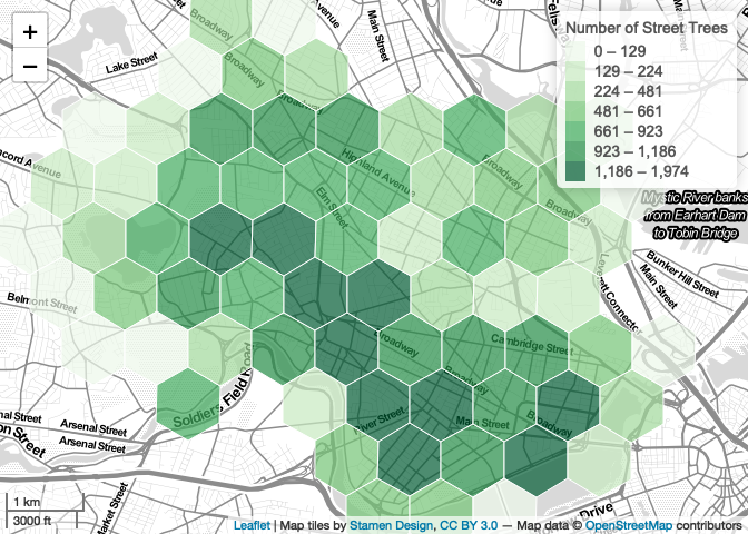

Simple interactivity tweaks like this encourage the map viewer to play, interact, and explore! But if we’re going to entice their further attention like this, we should at least give them a bit more information for their troubles… in addition to highlighing we can also add pop-up labels that print the tree count and hexagon id.

First, we create a list of labels—one for each hexagon! This code looks complicated, but let’s break it down… for each row, we use the stringr package’s str_glue function to create a string that includes both the value of trees and hex_id. In this string, we use HTML markup to indicate that we want XXX trees to be bold (<strong></strong>). Finally, we use lapply to mark each item in the list as HTML. This means that the HTML markup will not be displayed as text, but interpreted as HTML.

require('stringr')

labels <- str_glue("<strong>{hex$trees} trees</strong> in hexagon {hex$hex_id}") %>%
  lapply(htmltools::HTML)

We can then add this to our map like so:

map <- hex %>%
  leaflet() %>%
  setView(-71.111408, 42.38172, 13) %>%
  addProviderTiles("Stamen.TonerLite")  %>%
  addScaleBar(position='bottomleft') %>%
  addPolygons(
    fillColor = ~palette_quantiles(trees),
    fillOpacity = 0.7,
    opacity = 1,
    weight = 1,
    color='white',
    highlight = highlightOptions(
      weight = 3,
      bringToFront = TRUE),
    # Add labels here.
    label = labels
    ) %>%
  addLegend(
    title = "Number of Street Trees",
    pal = palette_quantiles,
    opacity = 0.7,
    values = trees,
    labFormat = labelFormat(
      digits = 0
    )
  )
map

# mapshot(m, url="output.html")

That’s it! We now have a map that displays additional information with user interaction… not too bad for a few lines of code, without ever leaving R!

Tidying Up

However, as we’ve made our map more interactive, you may have noticed some annoying features; it’s possible for the user to zoom out far further than would be useful in our application. The same can be said for panning: the user can pan around the world, potentially becoming quite lost. Finally, if you’re a person who’s done quite a bit of programming, it might be making you itch that we’ve hard-coded the setView latitude and longitude. Let’s deal with each one of these things in turn. First: setting a minimum zoom.

Set a Minimum Zoom

We can set a minimum zoom using the minZoom parameter of the leafletOptions function. When a minimum zoom is specified, the user will not be able to zoom out further than the minimum. Here, we set it to 12—one ‘step’ out from the default of 13. Simple enough!

map <- hex %>%
  leaflet(
    options = leafletOptions(
        minZoom = 12
      )
    ) %>%
  setView(-71.111408, 42.38172, 13) %>%
  addProviderTiles("Stamen.TonerLite")  %>%
  addScaleBar(position='bottomleft') %>%
  addPolygons(
    fillColor = ~palette_quantiles(trees),
    fillOpacity = 0.7,
    opacity = 1,
    weight = 1,
    color='white',
    highlight = highlightOptions(
      weight = 3,
      bringToFront = TRUE),
    # Add labels here.
    label = labels
    ) %>%
  addLegend(
    title = "Number of Street Trees",
    pal = palette_quantiles,
    opacity = 0.7,
    values = trees,
    labFormat = labelFormat(
      digits = 0
    )
  )
map

Bound the Map

In addition to ensuring that the user doesn’t have the ability to accidentally zoom out much farther than is useful, we may also want to put a fence around their horizontal panning. This is very useful—one of the more frustrating things when interacting with a map is dragging around, trying to find your starting point after an vigorous click-and-drag sends you sliding off into the world.

We set this using the setMaxBounds function, which takes four parameters: the latitude and longitude of the top-left corner of a bounding box, and the same for the bottom-right. We can programmatically generate these by simply using the bounding box of the hexagons, which are conveniently accessible to use using the st_bbox function.

bbox <- st_bbox(hex)
print(bbox)

##      xmin      ymin      xmax      ymax 
## -71.16930  42.34927 -71.06187  42.42051

We want to pass only the values, excluding their names, to the parameters of the setMaxBounds function—to the R user, this means using the double-bracket! Double-brackets allow you to access only values, stripping away names.

map <- hex %>%
  leaflet(
    options = leafletOptions(
        minZoom = 12
      )
    ) %>%
  setMaxBounds(
    lng1 = bbox[['xmin']],
    lat1 = bbox[['ymin']],
    lng2 = bbox[['xmax']],
    lat2 = bbox[['ymax']]
  ) %>%
  setView(-71.111408, 42.38172, 13) %>%
  addProviderTiles("Stamen.TonerLite")  %>%
  addPolygons(
    fillColor = ~palette_quantiles(trees),
    fillOpacity = 0.7,
    opacity = 1,
    weight = 1,
    color='white',
    highlight = highlightOptions(
      weight = 3,
      bringToFront = TRUE),
    label = labels
    ) %>%
  addLegend(
    title = "Number of Street Trees",
    pal = palette_quantiles,
    opacity = 0.7,
    values = trees,
    labFormat = labelFormat(
      digits = 0
    )
  )
map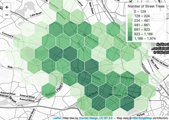

Setting MaxBounds makes interacting with and exploring your map much less frustrating for users.

Programmatically Center the Map

If you’re a person who does much programming, you may be bristling at the fact that we’re manually passing in latitudes and longitudes to the setView function. Instead, you might ask, isn’t there a way to set this programmatically based on the center of our dataset? Yes, dear reader, there is.

Let’s calculate the center of our dataset. First, we perform a union, which dissolves the edges between adjacent polygons, producing a single large polygon…

plot(st_union(hex))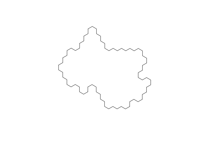

Next, we locate the centroid…

plot(st_union(hex))
plot(st_centroid(st_union(hex)), add=TRUE)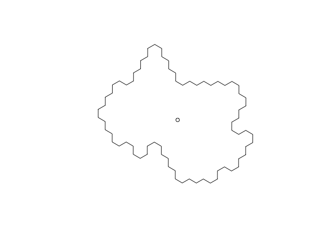

Finally, we pull out the coordinates of the centroid.

center <- st_coordinates(
  st_centroid(
    st_union(hex)
    )
  )
print(center)

##           X        Y
## 1 -71.11408 42.38172

These values can be passed to the setView function, instead of hard-coding them.

map <- hex %>%
  leaflet(
    options = leafletOptions(
        minZoom = 12
      )
    ) %>%
  setMaxBounds(
    lng1 = bbox[['xmin']],
    lat1 = bbox[['ymin']],
    lng2 = bbox[['xmax']],
    lat2 = bbox[['ymax']]
  ) %>%
  # Access x and y or center here...
  setView(center[,'X'], center[,'Y'], 13) %>%
  addProviderTiles("Stamen.TonerLite")  %>%
  addPolygons(
    fillColor = ~palette_quantiles(trees),
    fillOpacity = 0.7,
    opacity = 1,
    weight = 1,
    color='white',
    highlight = highlightOptions(
      weight = 3,
      bringToFront = TRUE),
    label = labels
    ) %>%
  addLegend(
    title = "Number of Street Trees",
    pal = palette_quantiles,
    opacity = 0.7,
    values = trees,
    labFormat = labelFormat(
      digits = 0
    )
  )
map

Exporting the Map

Once you’ve produced a map, you’ll probably want to export it. I do this using the mapshot package, which allows you to quickly and simply export a leaflet map object to either a ready-to-host HTML file, or a image (.png, .jpg, etc.).

require('mapshot')

## Loading required package: mapshot

## Warning in library(package, lib.loc = lib.loc, character.only = TRUE, logical.return = TRUE, : there is no package called 'mapshot'

# Export to an HTML file...
mapshot(map, url = "street_trees.html")
# Export to a image file...
mapshot(map, file = "street_trees.png")

When you first try to export your map, you may see this message:

PhantomJS not found. You can install it with webshot::install_phantomjs(). If it is installed, please make sure the phantomjs executable can be found via the PATH variable.

If you do, simply run webshot::install_phantomjs() (as directed)! Opening the html file in a web browser, you should see your map, as designed in R, ready to be hosted and displayed publicly!

References